10.1 Computing high symmetry molecules.

MOLCAS makes intensive use of the symmetry properties of the molecular systems in all parts of the calculation. The highest symmetry point group available, however, is the D_2h point group, which makes things somewhat more complicated when the molecule has higher symmetry. One of such cases is the calculation of linear molecules. In this section we describe calculations on different electronic states of three diatomic molecules: NiH, a heteronuclear molecule which belongs to the $C_{{\infty}v}$ symmetry group and C₂ and Ni₂, two homonuclear molecules which belong to the $D_{{\infty}h}$ symmetry group. They must be computed in MOLCAS using the lower order symmetry groups C_2v and D_2h, respectively, and therefore some codes such RASSCF use specific tools to constrain the resulting wave functions to have the higher symmetry of the actual point group. It must be pointed out clearly that linear symmetry cannot always be fully obtained in MOLCAS because the tools to average over degenerate representations are not totally implemented presently in the RASSCF program. This is the case, for instance, for the $\delta$ orbitals in a C_2v- $C_{{\infty}v}$ situation, as will be shown below. (For problems related to accurate calculations of diatomic molecules and symmetry see Ref. [238] and [239], respectively.). In a final section we will briefly comment the situation of high symmetry systems other than linear.

10.1.1 A diatomic heteronuclear molecule: NiH

Chemical bonds involving transition-metal atoms are often complex in nature due to the common presence of several unpaired electrons resulting in many close-lying spectroscopic states and a number of different factors such spin-orbit coupling or the importance of relativistic effects. NiH was the first system containing a transition-metal atom to be studied with the CASSCF method [240]. The large dynamic correlation effects inherent in a 3d semi-occupied shell with many electrons is a most severe problem, which few methods have been able to compute. The calculated dipole moment of the system has become one measurement of the quality of many ab initio methods [85]. We are not going to analyze the effects in detail. Let us only say that an accurate treatment of the correlation effects requires high quality methods such as MRCI, ACPF or CASPT2, large basis sets, and an appropriate treatment of relativistic effects, basis set superposition errors, and core-valence correlation. A detailed CASPT2 calculation of the ground state of NiH can be found elsewhere [241].

The ³F (3d⁸4s²) and ³D (3d⁹4s¹) states of the nickel atom are almost degenerate with a splitting of only 0.03 eV [242] and are characterized by quite different chemical behavior. In systems such as the $^2\Delta$ ground state of NiH molecule, where both states take part in the bonding, an accurate description of the low-lying Ni atomic states is required. The selection of the active space for NiH is not trivial. The smallest set of active orbitals for the $^2\Delta$ ground state which allows a proper dissociation and also takes into account the important $3d\sigma$ correlation comprises the singly occupied 3d_xy orbital and three $\sigma$ orbitals ( $3d_{z^2},\sigma,$ and $\sigma^*$ ). One cannot however expect to obtain accurate enough molecular properties just by including non-dynamical correlation effects. MRCI+Q calculations with the most important CASSCF configurations in the reference space proved that at least one additional $3d\delta$ (3d_x²-y²) and its correlating orbital were necessary to obtain spectroscopic constants in close agreement with the experimental values. It is, however, a larger active space comprising all the eleven valence electrons distributed in twelve active orbitals ( $\sigma,\sigma^*,d,d'$ ) that is the most consistent choice of active orbitals as evidenced in the calculation of other metal hydrides such as CuH [241] and in the electronic spectrum of the Ni atom [242]. This is the active space we are going to use in the following example. We will use the ANO-type basis set contracted to Ni [5s4p3d1f] / H [3s2p] for simplicity. In actual calculations g functions on the transition metal and d functions on the hydrogen atom are required to obtain accurate results.

First we need to know the behavior of each one of the basis functions within each one of the symmetries. Considering the molecule placed in the z axis the classification of the spherical harmonics into the $C_{{\infty}v}$ point group is:

**Table:** Classification of the spherical harmonics in the $C_{{\infty}v}$ group.
Symmetry	Spherical harmonics
$\sigma$	s	p_z	d_z²	f_z³
$\pi$	p_x	p_y	d_xz	d_yz	f_x(z²-y²)	f_y(z²-x²)
$\delta$	d_x²-y²	d_xy	f_xyz	f_z(x²-y²)
$\phi$	f_x³	f_y³

In C_2v, however, the functions are distributed into the four representations of the group and therefore different symmetry representations can be mixed. The next table lists the distribution of the functions in C_2v and the symmetry of the corresponding orbitals in $C_{{\infty}v}$ .

**Table:** Classification of the spherical harmonics and $C_{{\infty}v}$ orbitals in the C_2v group.
Symm.^a	Spherical harmonics (orbitals in $C_{{\infty}v}$ )
a₁ (1)	s ( $\sigma$ )	p_z ( $\sigma$ )	d_z² ( $\sigma$ )	d_x²-y² ( $\delta$ )	f_z³ ( $\sigma$ )	f_z(x²-y²) ( $\delta$ )
b₁ (2)	p_x ( $\pi$ )	d_xz ( $\pi$ )	f_x(z²-y²) ( $\pi$ )	f_x³ ( $\phi$ )
b₂ (3)	p_y ( $\pi$ )	d_yz ( $\pi$ )	f_y(z²-x²) ( $\pi$ )	f_y³ ( $\phi$ )
a₂ (4)	d_xy ( $\delta$ )	f_xyz ( $\delta$ )
^aIn parenthesis the number of the symmetry in MOLCAS. It depends on the generators used in `SEWARD`.

In symmetry ${\rm a}_1$ we find both $\sigma$ and $\delta$ orbitals. When the calculation is performed in C_2v symmetry all the orbitals of ${\rm a}_1$ symmetry can mix because they belong to the same representation, but this is not correct for $C_{{\infty}v}$ . The total symmetry must be kept $C_{{\infty}v}$ and therefore the $\delta$ orbitals should not be allowed to rotate and mix with the $\sigma$ orbitals. The same is true in the ${\rm b}_1$ and ${\rm b}_2$ symmetries with the $\pi$ and $\phi$ orbitals, while in ${\rm a}_2$ symmetry this problem does not exist because it has only $\delta$ orbitals (with a basis set up to f functions).

The tool to restrict possible orbital rotations is the option SUPSym in the RASSCF program. It is important to start with clean orbitals belonging to the actual symmetry, that is, without unwanted mixing.

But the problems with the symmetry are not solved with the SUPSym option only. Orbitals belonging to different components of a degenerate representation should also be equivalent. For example: the $\pi$ orbitals in ${\rm b}_1$ and ${\rm b}_2$ symmetries should have the same shape, and the same is true for the $\delta$ orbitals in ${\rm a}_1$ and ${\rm a}_2$ symmetries. This can only be partly achieved in the RASSCF code. The input option AVERage will average the density matrices for representations ${\rm b}_1$ and ${\rm b}_2$ ( $\pi$ and $\phi$ orbitals), thus producing equivalent orbitals. The present version does not, however, average the $\delta$ orbital densities in representations ${\rm a}_1$ and ${\rm a}_2$ (note that this problem does not occur for electronic states with an equal occupation of the two components of a degenerate set, for example $\Sigma$ states). A safe way to obtain totally symmetric orbitals is to reduce the symmetry to C₁ (or C_s in the homonuclear case) and perform a state-average calculation for the degenerate components.

We need an equivalence table to know the correspondence of the symbols for the functions in MOLCAS to the spherical harmonics (SH):

**Table 10.3:** MOLCAS labeling of the spherical harmonics.
MOLCAS	SH	MOLCAS	SH	MOLCAS	SH
1s	s	3d2+	d_x²-y²	4f3+	f_x³
2px	p_x	3d1+	d_xz	4f2+	f_z(x²-y²)
2pz	p_z	3d0	d_z²	4f1+	f_x(z²-y²)
2py	p_y	3d1-	d_yz	4f0	f_z³
		3d2-	d_xy	4f1-	f_y(z²-x²)
				4f2-	f_xyz
				4f3-	f_y³

We begin by performing a SCF calculation and analyzing the resulting orbitals. The employed bond distance is close to the experimental equilibrium bond length for the ground state [241]. Observe in the following SEWARD input that the symmetry generators, planes yz and xz, lead to a C_2v representation. In the SCF input we have used the option OCCNumbers which allows specification of occupation numbers other than 0 or 2. It is still the closed shell SCF energy functional which is optimized, so the obtained SCF energy has no physical meaning. However, the computed orbitals are somewhat better for open shell cases as NiH. The energy of the virtual orbitals is set to zero due to the use of the IVO option. The order of the orbitals may change in different computers and versions of the code.

&SEWARD Title NiH G.S Symmetry X Y Basis set Ni.ANO-L...5s4p3d1f. Ni 0.00000 0.00000 0.000000 Bohr End of basis Basis set H.ANO-L...3s2p. H 0.000000 0.000000 2.747000 Bohr End of basis End of Input &SCF TITLE NiH G.S. OCCUPIED 8 3 3 1 OCCNumber 2.0 2.0 2.0 2.0 2.0 2.0 2.0 2.0 2.0 2.0 2.0 2.0 2.0 2.0 1.0

SCF orbitals + arbitrary occupations ~ Molecular orbitals for symmetry species 1 ~ ORBITAL 4 5 6 7 8 9 10 ENERGY -4.7208 -3.1159 -.5513 -.4963 -.3305 .0000 .0000 OCC. NO. 2.0000 2.0000 2.0000 2.0000 2.0000 .0000 .0000 ~ 1 NI 1s0 .0000 .0001 .0000 -.0009 .0019 .0112 .0000 2 NI 1s0 .0002 .0006 .0000 -.0062 .0142 .0787 .0000 3 NI 1s0 1.0005 -.0062 .0000 -.0326 .0758 .3565 .0000 4 NI 1s0 .0053 .0098 .0000 .0531 -.4826 .7796 .0000 5 NI 1s0 -.0043 -.0032 .0000 .0063 -.0102 -.0774 .0000 6 NI 2pz .0001 .0003 .0000 -.0015 .0029 .0113 .0000 7 NI 2pz -.0091 -.9974 .0000 -.0304 .0622 .1772 .0000 8 NI 2pz .0006 .0013 .0000 .0658 -.1219 .6544 .0000 9 NI 2pz .0016 .0060 .0000 .0077 -.0127 -.0646 .0000 10 NI 3d0 -.0034 .0089 .0000 .8730 .4270 .0838 .0000 11 NI 3d0 .0020 .0015 .0000 .0068 .0029 .8763 .0000 12 NI 3d0 .0002 .0003 .0000 -.0118 -.0029 -.7112 .0000 13 NI 3d2+ .0000 .0000 -.9986 .0000 .0000 .0000 .0175 14 NI 3d2+ .0000 .0000 .0482 .0000 .0000 .0000 .6872 15 NI 3d2+ .0000 .0000 .0215 .0000 .0000 .0000 -.7262 16 NI 4f0 .0002 .0050 .0000 -.0009 -.0061 .0988 .0000 17 NI 4f2+ .0000 .0000 .0047 .0000 .0000 .0000 -.0033 18 H 1s0 -.0012 -.0166 .0000 .3084 -.5437 -.9659 .0000 19 H 1s0 -.0008 -.0010 .0000 -.0284 -.0452 -.4191 .0000 20 H 1s0 .0014 .0007 .0000 .0057 .0208 .1416 .0000 21 H 2pz .0001 .0050 .0000 -.0140 .0007 .5432 .0000 22 H 2pz .0008 -.0006 .0000 .0060 -.0093 .2232 .0000 ~ ORBITAL 11 12 13 14 15 16 18 ENERGY .0000 .0000 .0000 .0000 .0000 .0000 .0000 OCC. NO. .0000 .0000 .0000 .0000 .0000 .0000 .0000 ~ 1 NI 1s0 -.0117 -.0118 .0000 .0025 .0218 -.0294 .0000 2 NI 1s0 -.0826 -.0839 .0000 .0178 .1557 -.2087 .0000 3 NI 1s0 -.3696 -.3949 .0000 .0852 .7386 -.9544 .0000 4 NI 1s0 -1.3543 -1.1537 .0000 .3672 2.3913 -2.8883 .0000 5 NI 1s0 -.3125 .0849 .0000 -1.0844 .3670 -.0378 .0000 6 NI 2pz -.0097 -.0149 .0000 .0064 .0261 -.0296 .0000 7 NI 2pz -.1561 -.2525 .0000 .1176 .4515 -.4807 .0000 8 NI 2pz -.3655 -1.0681 .0000 .0096 1.7262 -2.9773 .0000 9 NI 2pz -1.1434 -.0140 .0000 -.1206 .2437 -.9573 .0000 10 NI 3d0 -.1209 -.2591 .0000 .2015 .5359 -.4113 .0000 11 NI 3d0 -.3992 -.3952 .0000 .1001 .3984 -.9939 .0000 12 NI 3d0 -.1546 -.1587 .0000 -.1676 -.2422 -.4852 .0000 13 NI 3d2+ .0000 .0000 -.0048 .0000 .0000 .0000 -.0498 14 NI 3d2+ .0000 .0000 -.0017 .0000 .0000 .0000 -.7248 15 NI 3d2+ .0000 .0000 .0028 .0000 .0000 .0000 -.6871 16 NI 4f0 -.1778 -1.0717 .0000 -.0233 .0928 -.0488 .0000 17 NI 4f2+ .0000 .0000 -1.0000 .0000 .0000 .0000 -.0005 18 H 1s0 1.2967 1.5873 .0000 -.3780 -2.7359 3.8753 .0000 19 H 1s0 1.0032 .4861 .0000 .3969 -.9097 1.8227 .0000 20 H 1s0 -.2224 -.2621 .0000 .1872 .0884 -.7173 .0000 21 H 2pz -.1164 -.4850 .0000 .3388 1.1689 -.4519 .0000 22 H 2pz -.1668 -.0359 .0000 .0047 .0925 -.3628 .0000 ~ Molecular orbitals for symmetry species 2 ~ ORBITAL 2 3 4 5 6 7 ENERGY -3.1244 -.5032 .0000 .0000 .0000 .0000 OCC. NO. 2.0000 2.0000 .0000 .0000 .0000 .0000 ~ 1 NI 2px -.0001 .0001 .0015 .0018 .0012 -.0004 2 NI 2px -.9999 .0056 .0213 .0349 .0235 -.0054 3 NI 2px -.0062 -.0140 .1244 -.3887 .2021 -.0182 4 NI 2px .0042 .0037 .0893 .8855 -.0520 .0356 5 NI 3d1+ .0053 .9993 .0268 .0329 .0586 .0005 6 NI 3d1+ -.0002 -.0211 -.5975 .1616 .1313 .0044 7 NI 3d1+ -.0012 -.0159 .7930 .0733 .0616 .0023 8 NI 4f1+ .0013 -.0049 .0117 .1257 1.0211 -.0085 9 NI 4f3+ -.0064 .0000 -.0003 -.0394 .0132 .9991 10 H 2px -.0008 .0024 -.0974 -.1614 -.2576 -.0029 11 H 2px .0003 -.0057 -.2060 -.2268 -.0768 -.0079 ~ Molecular orbitals for symmetry species 3 ~ ORBITAL 2 3 4 5 6 7 ENERGY -3.1244 -.5032 .0000 .0000 .0000 .0000 OCC. NO. 2.0000 2.0000 .0000 .0000 .0000 .0000 ~ 1 NI 2py -.0001 .0001 -.0015 .0018 .0012 .0004 2 NI 2py -.9999 .0056 -.0213 .0349 .0235 .0054 3 NI 2py -.0062 -.0140 -.1244 -.3887 .2021 .0182 4 NI 2py .0042 .0037 -.0893 .8855 -.0520 -.0356 5 NI 3d1- .0053 .9993 -.0268 .0329 .0586 -.0005 6 NI 3d1- -.0002 -.0211 .5975 .1616 .1313 -.0044 7 NI 3d1- -.0012 -.0159 -.7930 .0733 .0616 -.0023 8 NI 4f3- .0064 .0000 -.0003 .0394 -.0132 .9991 9 NI 4f1- .0013 -.0049 -.0117 .1257 1.0211 .0085 10 H 2py -.0008 .0024 .0974 -.1614 -.2576 .0029 11 H 2py .0003 -.0057 .2060 -.2268 -.0768 .0079 ~ Molecular orbitals for symmetry species 4 ~ ORBITAL 1 2 3 4 ENERGY -.0799 .0000 .0000 .0000 OCC. NO. 1.0000 .0000 .0000 .0000 ~ 1 NI 3d2- -.9877 -.0969 .0050 -.1226 2 NI 3d2- -.1527 .7651 .0019 .6255 3 NI 3d2- -.0332 -.6365 -.0043 .7705 4 NI 4f2- .0051 -.0037 1.0000 .0028

In difficult situations it can be useful to employ the AUFBau option of the SCF program. Including this option, the subsequent classification of the orbitals in the different symmetry representations can be avoided. The program will look for the lowest-energy solution and will provide with a final occupation. This option must be used with caution. It is only expected to work in clear closed-shell situations.

We have only printed the orbitals most relevant to the following discussion. Starting with symmetry 1 ( ${\rm a}_1$ ) we observe that the orbitals are not mixed at all. Using a basis set contracted to Ni 5s4p3d1f / H 3s2p in symmetry ${\rm a}_1$ we obtain 18 $\sigma$ molecular orbitals (combinations from eight atomic s functions, six p_z functions, three d_z² functions, and one f_z³ function) and four $\delta$ orbitals (from three d_x²-y² functions and one f_z(x²-y²) function). Orbitals 6, 10, 13, and 18 are formed by contributions from the three d_x²-y² and one f_z(x²-y²) $\delta$ functions, while the contributions of the remaining harmonics are zero. These orbitals are $\delta$ orbitals and should not mix with the remaining ${\rm a}_1$ orbitals. The same situation occurs in symmetries ${\rm b}_1$ and ${\rm b}_2$ (2 and 3) but in this case we observe an important mixing among the orbitals. Orbitals 7 ${\rm b}_1$ and 7 ${\rm b}_2$ have main contributions from the harmonics 4f3+ (f_x³) and 4f3- (f_y³), respectively. They should be pure $\phi$ orbitals and not mix at all with the remaining $\pi$ orbitals.

The first step is to evaluate the importance of the mixings for future calculations. Strictly, any kind of mixing should be avoided. If g functions are used, for instance, new contaminations show up. But, undoubtedly, not all mixings are going to be equally important. If the rotations occur among occupied or active orbitals the influence on the results is going to be larger than if they are high secondary orbitals. NiH is one of these cases. The ground state of the molecule is $^2\Delta$ . It has two components and we can therefore compute it by placing the single electron in the d_xy orbital (leading to a state of ${\rm a}_2$ symmetry in C_2v) or in the d_x²-y² orbital of the ${\rm a}_1$ symmetry. Both are $\delta$ orbitals and the resulting states will have the same energy provided that no mixing happens. In the ${\rm a}_2$ symmetry no mixing is possible because it is only composed of $\delta$ orbitals but in ${\rm a}_1$ symmetry the $\sigma$ and $\delta$ orbitals can rotate. It is clear that this type of mixing will be more important for the calculation than the mixing of $\pi$ and $\phi$ orbitals. However it might be necessary to prevent it. Because in the SCF calculation no high symmetry restriction was imposed on the orbitals, orbitals 2 and 4 of the ${\rm b}_1$ and ${\rm b}_2$ symmetries have erroneous contributions of the 4f3+ and 4f3- harmonics, and they are occupied or active orbitals in the following CASSCF calculation.

To use the supersymmetry (SUPSym) option we must start with proper orbitals. In this case the ${\rm a}_1$ orbitals are symmetry adapted (within the printed accuracy) but not the ${\rm b}_1$ and ${\rm b}_2$ orbitals. Orbitals 7 ${\rm b}_1$ and 7 ${\rm b}_2$ must have zero coefficients for all the harmonics except for 4f3+ and 4f3-, respectively. The remaining orbitals of these symmetries (even those not shown) must have zero in the coefficients corresponding to 4f3+ or 4f3-. To clean the orbitals the option CLEAnup of the RASSCF program can be used.

Once the orbitals are properly symmetrized we can perform CASSCF calculations on different electronic states. Deriving the types of the molecular electronic states resulting from the electron configurations is not simple in many cases. In general, for a given electronic configuration several electronic states of the molecule will result. Wigner and Witmer derived rules for determining what types of molecular states result from given states of the separated atoms. In chapter VI of reference [243] it is possible to find the tables of the resulting electronic states once the different couplings and the Pauli principle have been applied.

In the present CASSCF calculation we have chosen the active space (3d, 4d, $\sigma$ , $\sigma^*$ ) with all the 11 valence electrons active. If we consider 4d and $\sigma^*$ as weakly occupied correlating orbitals, we are left with 3d and $\sigma$ (six orbitals), which are to be occupied with 11 electrons. Since the bonding orbital $\sigma$ (composed mainly of Ni 4s and H 1s) will be doubly occupied in all low lying electronic states, we are left with nine electrons to occupy the 3d orbitals. There is thus one hole, and the possible electronic states are: $^2\Sigma^+$ , $^2\Pi$ , and $^2\Delta$ , depending on the orbital where the hole is located. Taking Table

into account we observe that we have two low-lying electronic states in symmetry 1 (A₁): $^2\Sigma^+$ and $^2\Delta$ , and one in each of the other three symmetries: $^2\Pi$ in symmetries 2 (B₁) and 3 (B₂), and $^2\Delta$ in symmetry 4 (A₂). It is not immediately obvious which of these states is the ground state as they are close in energy. It may therefore be necessary to study all of them. It has been found at different levels of theory that the NiH has a $^2\Delta$ ground state [241].

We continue by computing the $^2\Delta$ ground state. The previous SCF orbitals will be the initial orbitals for the CASSCF calculation. First we need to know in which C_2v symmetry or symmetries we can compute a $\Delta$ state. In the symmetry tables it is determined how the species of the linear molecules are resolved into those of lower symmetry (depends also on the orientation of the molecule). In Table

is listed the assignment of the different symmetries for the molecule placed on the z axis.

The $\Delta$ state has two degenerate components in symmetries ${\rm a}_1$ and ${\rm a}_2$ . Two CASSCF calculations can be performed, one computing the first root of ${\rm a}_2$ symmetry and the second for the first root of ${\rm a}_1$ symmetry. The RASSCF input for the state of ${\rm a}_2$ symmetry would be:

&RASSCF &END Title NiH 2Delta CAS s, s*, 3d, 3d'. Symmetry 4 Spin 2 Nactel 11 0 0 Inactive 5 2 2 0 Ras2 6 2 2 2 Thrs 1.0E-07,1.0E-05,1.0E-05 Cleanup 1 4 6 10 13 18 18 1 2 3 4 5 6 7 8 9 10 11 12 16 18 19 20 21 22 4 13 14 15 17 1 1 7 10 1 2 3 4 5 6 7 8 10 11 1 9 1 1 7 10 1 2 3 4 5 6 7 9 10 11 1 8 0 Supsym 1 4 6 10 13 18 1 1 7 1 1 7 0 *Average *1 2 3 Iter 50,25 LumOrb End of Input

The corresponding input for symmetry ${\rm a}_1$ will be identical except for the SYMMetry keyword
Symmetry 1

**Table:** Resolution of the $C_{{\infty}v}$ species in the C_2v species.
State symmetry $C_{{\infty}v}$		State symmetry C_2v
$\Sigma^+$		A₁
$\Sigma^-$		A₂
$\Pi$		B₁ + B₂
$\Delta$		A₁ + A₂
$\Phi$		B₁ + B₂
$\Gamma$		A₁ + A₂

In the RASSCF inputs the CLEAnup option will take the initial orbitals (SCF here) and will place zeroes in all the coefficients of orbitals 6, 10, 13, and 18 in symmetry 1, except in coefficients 13, 14, 15, and 17. Likewise all coefficients 13, 14, 15, and 17 of the remaining ${\rm a}_1$ orbitals will be set to zero. The same procedure is used in symmetries ${\rm b}_1$ and ${\rm b}_2$ . Once cleaned, and because of the SUPSymmetry option, the $\delta$ orbitals 6, 10, 13, and 18 of ${\rm a}_1$ symmetry will only rotate among themselves and they will not mix with the remaining ${\rm a}_1$ $\sigma$ orbitals. The same holds true for $\phi$ orbitals 7 ${\rm b}_1$ and 7 ${\rm b}_2$ in their respective symmetries.

Orbitals can change order during the calculation. MOLCAS incorporates a procedure to check the nature of the orbitals in each iteration. Therefore the right behavior of the SUPSym option is guaranteed during the calculation. The procedure can have problems if the initial orbitals are not symmetrized properly. Therefore, the output with the final results should be checked to compare the final order of the orbitals and the final labeling of the SUPSym matrix.

The AVERage option would average the density matrices of symmetries 2 and 3, corresponding to the $\Pi$ and $\Phi$ symmetries in $C_{{\infty}v}$ . In this case it is not necessary to use the option because the two components of the degenerate sets in symmetries ${\rm b}_1$ and ${\rm b}_2$ have the same occupation and therefore they will have the same shape. The use of the option in a situation like this ( $^2\Delta$ and $^2\Sigma^+$ states) leads to convergence problems. The symmetry of the orbitals in symmetries 2 and 3 is retained even if the AVERage option is not used.

The output for the calculation on symmetry 4 ( ${\rm a}_2$ ) contains the following lines:

Convergence after 29 iterations 30 2 2 1 -1507.59605678 -.23E-11 3 9 1 -.68E-06 -.47E-05 ~ Wave function printout: occupation of active orbitals, and spin coupling of open shells (u,d: Spin up or down) ~ printout of CI-coefficients larger than .05 for root 1 energy= -1507.596057 conf/sym 111111 22 33 44 Coeff Weight 15834 222000 20 20 u0 .97979 .95998 15838 222000 ud ud u0 .05142 .00264 15943 2u2d00 ud 20 u0 -.06511 .00424 15945 2u2d00 20 ud u0 .06511 .00424 16212 202200 20 20 u0 -.05279 .00279 16483 u220d0 ud 20 u0 -.05047 .00255 16485 u220d0 20 ud u0 .05047 .00255 ~ Natural orbitals and occupation numbers for root 1 sym 1: 1.984969 1.977613 1.995456 .022289 .014882 .005049 sym 2: 1.983081 .016510 sym 3: 1.983081 .016510 sym 4: .993674 .006884

The state is mainly (weight 96%) described by a single configuration (configuration number 15834) which placed one electron on the first active orbital of symmetry 4 ( ${\rm a}_2$ ) and the remaining electrons are paired. A close look to this orbital indicates that is has a coefficient -.9989 in the first 3d2- (3d_xy) function and small coefficients in the other functions. This results clearly indicate that we have computed the $^2\Delta$ state as the lowest root of that symmetry. The remaining configurations have negligible contributions. If the orbitals are properly symmetrized, all configurations will be compatible with a $^2\Delta$ electronic state.

Convergence after 15 iterations 16 2 3 1 -1507.59605678 -.19E-10 8 15 1 .35E-06 -.74E-05 ~ Wave function printout: occupation of active orbitals, and spin coupling of open shells (u,d: Spin up or down) ~ printout of CI-coefficients larger than .05 for root 1 energy= -1507.596057 conf/sym 111111 22 33 44 Coeff Weight 40800 u22000 20 20 20 -.97979 .95998 42400 u02200 20 20 20 .05280 .00279 ~ Natural orbitals and occupation numbers for root 1 sym 1: .993674 1.977613 1.995456 .022289 .006884 .005049 sym 2: 1.983081 .016510 sym 3: 1.983081 .016510 sym 4: 1.984969 .014882

We obtain the same energy as in the previous calculation. Here the dominant configuration places one electron on the first active orbital of symmetry 1 ( ${\rm a}_1$ ). It is important to remember that the orbitals are not ordered by energies or occupations into the active space. This orbital has also the coefficient -.9989 in the first 3d2- (3d_x²-y²) function. We have then computed the other component of the $^2\Delta$ state. As the $\delta$ orbitals in different C_2v symmetries are not averaged by the program it could happen (not in the present case) that the two energies differ slightly from each other.

The consequences of not using the SUPSym option are not extremely severe in the present example. If you perform a calculation without the option, the obtained energy is:

Convergence after 29 iterations 30 2 2 1 -1507.59683719 -.20E-11 3 9 1 -.69E-06 -.48E-05

As it is a broken symmetry solution the energy is lower than in the other case. This is a typical behavior. If we were using an exact wave function it would have the right symmetry properties, but approximated wave functions do not necessarily fulfill this condition. So, more flexibility leads to lower energy solutions which have broken the orbital symmetry.

If in addition to the $^2\Delta$ state we want to compute the lowest $^2\Sigma^+$ state we can use the adapted orbitals from any of the $^2\Delta$ state calculations and use the previous RASSCF input without the CLEAnup option. The orbitals have not changed place in this example. If they do, one has to change the labels in the SUPSym option. The simplest way to compute the lowest excited $^2\Sigma^+$ state is having the unpaired electron in one of the $\sigma$ orbitals because none of the other configurations, $\delta^3$ or $\pi^3$ , leads to the $^2\Sigma^+$ term. However, there are more possibilities such as the configuration $\sigma^1$ $\sigma^1$ $\sigma^1$ ; three nonequivalent electrons in three $\sigma$ orbitals. In actuality the lowest $^2\Sigma^+$ state must be computed as a doublet state in symmetry A₁. Therefore, we set the symmetry in the RASSCF to 1 and compute the second root of the symmetry (the first was the $^2\Delta$ state):

Of course the SUPSym option must be maintained. The use of CIROot indicates that we are computing the second root of that symmetry. The obtained result:

Convergence after 33 iterations 9 2 3 2 -1507.58420263 -.44E-10 2 11 2 -.12E-05 .88E-05 ~ Wave function printout: occupation of active orbitals, and spin coupling of open shells (u,d: Spin up or down) ~ printout of CI-coefficients larger than .05 for root 1 energy= -1507.584813 conf/sym 111111 22 33 44 Coeff Weight 40800 u22000 20 20 20 -.97917 .95877 ~ printout of CI-coefficients larger than .05 for root 2 energy= -1507.584203 conf/sym 111111 22 33 44 Coeff Weight 40700 2u2000 20 20 20 .98066 .96169 ~ Natural orbitals and occupation numbers for root 2 sym 1: 1.983492 .992557 1.995106 .008720 .016204 .004920 sym 2: 1.983461 .016192 sym 3: 1.983451 .016192 sym 4: 1.983492 .016204

As we have used two as the dimension of the CI matrix employed in the CI Davidson procedure we obtain the wave function of two roots, although the optimized root is the second. Root 1 places one electron in the first active orbital of symmetry one, which is a 3d2+ (3d_x²-y²) $\delta$ orbital. Root 2 places the electron in the second active orbital, which is a $\sigma$ orbital with a large coefficient (.9639) in the first 3d0 (3d_z²) function of the nickel atom. We have therefore computed the lowest $^2\Sigma^+$ state. The two $^2\Sigma^+$ states resulting from the configuration with the three unpaired $\sigma$ electrons is higher in energy at the CASSCF level. If the second root of symmetry ${\rm a}_1$ had not been a $^2\Sigma^+$ state we would have to study higher roots of the same symmetry.

It is important to remember that the active orbitals are not ordered at all within the active space. Therefore, their order might vary from calculation to calculation and, in addition, no conclusions about the orbital energy, occupation or any other information can be obtained from the order of the active orbitals.

We can compute also the lowest $^2\Pi$ excited state. The simplest possibility is having the configuration $\pi^3$ , which only leads to one $^2\Pi$ state. The unpaired electron will be placed in either one ${\rm b}_1$ or one ${\rm b}_2$ orbital. That means that the state has two degenerate components and we can compute it equally in both symmetries. There are more possibilities, such as the configuration $\pi^3\sigma^1\sigma^1$ or the configuration $\pi^3\sigma^1\delta^1$ . The resulting $^2\Pi$ state will always have two degenerate components in symmetries ${\rm b}_1$ and ${\rm b}_2$ , and therefore it is the wave function analysis which gives us the information of which configuration leads to the lowest $^2\Pi$ state.

For NiH it turns out to be non trivial to compute the $^2\Pi$ state. Taking as initial orbitals the previous SCF orbitals and using any type of restriction such as the CLEAnup, SUPSym or AVERage options lead to severe convergence problems like these:

45 9 17 1 -1507.42427683 -.65E-02 6 18 1 -.23E-01 -.15E+00 46 5 19 1 -1507.41780710 .65E-02 8 15 1 .61E-01 -.15E+00 47 9 17 1 -1507.42427683 -.65E-02 6 18 1 -.23E-01 -.15E+00 48 5 19 1 -1507.41780710 .65E-02 8 15 1 .61E-01 -.15E+00 49 9 17 1 -1507.42427683 -.65E-02 6 18 1 -.23E-01 -.15E+00 50 5 19 1 -1507.41780710 .65E-02 8 15 1 .61E-01 -.15E+00 ~ No convergence after 50 iterations 51 9 19 1 -1507.42427683 -.65E-02 6 18 1 -.23E-01 -.15E+00

The calculation, however, converges in an straightforward way if none of those tools are used:

Convergence after 33 iterations 34 2 2 1 -1507.58698677 -.23E-12 3 8 2 -.72E-06 -.65E-05 ~ Wave function printout: occupation of active orbitals, and spin coupling of open shells (u,d: Spin up or down) ~ printout of CI-coefficients larger than .05 for root 1 energy= -1507.586987 conf/sym 111111 22 33 44 Coeff Weight 15845 222000 u0 20 20 .98026 .96091 15957 2u2d00 u0 ud 20 .05712 .00326 16513 u220d0 u0 20 ud -.05131 .00263 ~ Natural orbitals and occupation numbers for root 1 sym 1: 1.984111 1.980077 1.995482 .019865 .015666 .004660 sym 2: .993507 .007380 sym 3: 1.982975 .016623 sym 4: 1.983761 .015892

The $\pi$ (and $\phi$ ) orbitals, both in symmetries ${\rm b}_1$ and ${\rm b}_2$ , are, however, differently occupied and therefore are not equal as they should be:

Molecular orbitals for sym species 2 Molecular orbitals for symmetry species 3 ORBITAL 3 4 ORBITAL 3 4 ENERGY .0000 .0000 ENERGY .0000 .0000 OCC. NO. .9935 .0074 OCC. NO. 1.9830 .0166 ~ 1 NI 2px .0001 .0002 1 NI 2py .0018 -.0001 2 NI 2px .0073 .0013 2 NI 2py .0178 -.0002 3 NI 2px -.0155 .0229 3 NI 2py -.0197 -.0329 4 NI 2px .0041 .0227 4 NI 2py .0029 -.0254 5 NI 3d1+ .9990 -.0199 5 NI 3d1- .9998 -.0131 6 NI 3d1+ -.0310 -.8964 6 NI 3d1- .0128 .9235 7 NI 3d1+ -.0105 .4304 7 NI 3d1- .0009 -.3739 8 NI 4f1+ -.0050 .0266 8 NI 4f3- .0001 -.0003 9 NI 4f3+ .0001 .0000 9 NI 4f1- -.0050 -.0177 10 H 2px .0029 -.0149 10 H 2py .0009 .0096 11 H 2px -.0056 -.0003 11 H 2py -.0094 -.0052

Therefore what we have is a symmetry broken solution. To obtain a solution which is not of broken nature the $\pi$ and $\phi$ orbitals must be equivalent. The tool to obtain equivalent orbitals is the AVERage option, which averages the density matrices of symmetries ${\rm b}_1$ and ${\rm b}_2$ . But starting with any of the preceding orbitals and using the AVERage option lead again to convergence problems. It is necessary to use better initial orbitals; orbitals which have already equal orbitals in symmetries ${\rm b}_1$ and ${\rm b}_2$ . One possibility is to perform a SCF calculation on the NiH cation explicitly indicating occupation one in the two higher occupied $\pi$ orbitals (symmetries 2 and 3):

&SCF &END TITLE NiH cation OCCUPIED 8 3 3 1 OCCNO 2.0 2.0 2.0 2.0 2.0 2.0 2.0 2.0 2.0 2.0 1.0 <-- Note the extra occupation 2.0 2.0 1.0 <-- Note the extra occupation 2.0 IVO END OF INPUT

It can take some successive steps to obtain a converged calculation using the CLEAnup, SUPSym, and AVERage options. The calculation with a single root did not converge clearly. We obtained, however, a converged result for the lowest $^2\Pi$ state of NiH by computing two averaged CASSCF roots and setting a weight of 90% for the first root using the keyword:

~ Wave function printout: occupation of active orbitals, and spin coupling of open shells (u,d: Spin up or down) ~ printout of CI-coefficients larger than .05 for root 1 energy= -1507.566492 conf/sym 111111 22 33 44 Coeff Weight 4913 222u00 20 d0 u0 -.05802 .00337 15845 222000 u0 20 20 .97316 .94703 15953 2u2d00 u0 20 20 .05763 .00332 16459 2u20d0 u0 20 ud -.05283 .00279 ~ Natural orbitals and occupation numbers for root 1 sym 1: 1.972108 1.982895 1.998480 .028246 .016277 .007159 sym 2: .997773 .007847 sym 3: 1.978019 .016453 sym 4: 1.978377 .016366

The energy of the different states (only the first one shown above) is printed on the top of their configuration list. The converged energy is simply an average energy. The occupation numbers obtained in the section of the RASSCF output printed above are the occupation numbers of the natural orbitals of the corresponding root. They differ from the occupation numbers printed in the molecular orbital section where we have pseudonatural molecular orbitals and average occupation numbers. On top of each of the valence $\pi$ orbitals an average occupation close to 1.5e will be printed; this is a consequence of the the averaging procedure.

The results obtained are only at the CASSCF level. Additional effects have to be considered and included. The most important of them is the dynamical correlation effect which can be added by computing, for instance, the CASPT2 energies. The reader can find a detailed explanation of the different approaches in ref. [241], and a careful discussion of their consequences and solutions in ref. [244].

We are going, however, to point out some details. In the first place the basis set must include up to g functions for the transition metal atom and up to d functions for the hydrogen. Relativistic effects must be taken into account, at least in a simple way as a first order correction. The keyword RELInt must be then included in the SEWARD input to compute the mass-velocity and one-electron Darwin contact term integrals and obtain a first-order correction to the energy with respect to relativistic effects at the CASSCF level in the RASSCF output. Scalar relativistic effects can be also included according the Douglas-Kroll or the Barysz-Sadlej-Snijders transformations, as it will be explained in section

The CASPT2 input needed to compute the second-order correction to the energy will include the number of the CASSCF root to compute. For instance, for the first root of each symmetry:

The number of frozen orbitals taken by CASPT2 will be that specified in the RASSCF input except if this is changed in the CASPT2 input. In the perturbative step we have frozen all the occupied orbitals except the active ones. This is motivated by the desire to include exclusively the dynamical correlation related to the valence electrons. In this way we neglect correlation between core electrons, named core-core correlation, and between core and valence electrons, named core-valence correlation. This is not because the calculation is smaller but because of the inclusion of those type of correlation in a calculation designed to treat valence correlation is an inadequate approach. Core-core and core-valence correlation requires additional basis functions of the same spatial extent as the occupied orbitals being correlated, but with additional radial and angular nodes. Since the spatial extent of the core molecular orbitals is small, the exponents of these correlating functions must be much larger than those of the valence optimized basis sets. The consequence is that we must avoid the inclusion of the core electrons in the treatment in the first step. Afterwards, the amount of correlation introduced by the core electrons can be estimated in separated calculations for the different states and those effects added to the results with the valence electrons.

Core-valence correlation effects of the 3s and 3p nickel shells can be studied by increasing the basis set flexibility by uncontracting the basis set in the appropriate region. There are different possibilities. Here we show the increase of the basis set by four s, four p, and four d functions. f functions contribute less to the description of the 3s and 3p shells and can be excluded. The uncontracted exponents should correspond to the region where the 3s and 3p shells present their density maximum. Therefore, first we compute the absolute maxima of the radial distribution of the involved orbitals, then we determine the primitive gaussian functions which have their maxima in the same region as the orbitals and therefore which exponents should be uncontracted. The final basis set will be the valence basis set used before plus the new added functions. In the present example the SEWARD input can be:

&SEWARD &END Title NiH G.S. Symmetry X Y *RelInt Basis set Ni.ANO-L...5s4p3d1f. Ni 0.00000 0.00000 0.000000 Bohr End of basis Basis set Ni....4s4p4d. / Inline 0. 2 * Additional s functions 4 4 3.918870 1.839853 0.804663 0.169846 1. 0. 0. 0. 0. 1. 0. 0. 0. 0. 1. 0. 0. 0. 0. 1. * Additional p functions 4 4 2.533837 1.135309 0.467891 0.187156 1. 0. 0. 0. 0. 1. 0. 0. 0. 0. 1. 0. 0. 0. 0. 1. * Additional d functions 4 4 2.551303 1.128060 0.475373 0.182128 1. 0. 0. 0. 0. 1. 0. 0. 0. 0. 1. 0. 0. 0. 0. 1. Nix 0.00000 0.00000 0.000000 Bohr End of basis Basis set H.ANO-L...3s2p. H 0.000000 0.000000 2.747000 Bohr End of basis End of Input

We have used a special format to include the additional functions. We include the additional 4s4p4d functions for the nickel atom. The additional basis set input must use a dummy label (Nix here), the same coordinates of the original atom, and specify a CHARge equal to zero, whether in an Inline basis set input as here or by specifically using keyword CHARge. It is not necessary to include the basis set with the Inline format. A library can be created for this purpose. In this case the label for the additional functions could be:

and a proper link to AUXLIB should be included in the script (or in the input if one uses AUTO).

Now the CASPT2 is going to be different to include also the correlation related to the 3s,3p shell of the nickel atom. Therefore, we only freeze the 1s,2s,2p shells:

&CASPT2 &END Title NiH. Core-valence. Frozen 3 1 1 0 Maxit 30 Lroot 1 End of input

A final effect one should study is the basis set superposition error (BSSE). In many cases it is a minor effect but it is an everpresent phenomenon which should be investigated when high accuracy is required, especially in determining bond energies, and not only in cases with weakly interacting systems, as is frequently believed. The most common approach to estimate this effect is the counterpoise correction: the separated fragment energies are computed in the total basis set of the system. For a discussion of this issue see Refs. [244,245]. In the present example we would compute the energy of the isolated nickel atom using a SEWARD input including the full nickel basis set plus the hydrogen basis set in the hydrogen position but with the charge set to zero. And then the opposite should be done to compute the energy of isolated hydrogen. The BSSE depends on the separation of the fragments and must be estimated at any computed geometry. For instance, the SEWARD input necessary to compute the isolated hydrogen atom at a given distance from the ghost nickel basis set including core uncontracted functions is:

>>UNIX mkdir AUXLIB >>COPY $CurrDir/NiH.NewLib AUXLIB/UNCONTRACTED &SEWARD &END Title NiH. 3s3p + H (BSSE) Symmetry X Y RelInt Basis set Ni.ANO-L...5s4p3d1f. Ni 0.00000 0.00000 0.000000 Bohr Charge 0.0 End of basis Basis set Ni.Uncontracted...4s4p4d. / AUXLIB Nix 0.00000 0.00000 0.000000 Bohr Charge 0.0 End of basis Basis set H.ANO-L...3s2p. H 0.000000 0.000000 2.747000 Bohr End of basis End of Input Once the energy of each of the fragments with the corresponding ghost basis set of the other fragment is determined, the energies of the completely isolated fragments can be computed and subtracted from those which have the ghost basis sets. Other approaches used to estimate the BSSE effect are discussed in Ref. [244].

The results obtained at the CASPT2 level are close to those obtained by MRCI+Q and ACPF treatments but more accurate. They match well with experiment. The difference is that all the configuration functions (CSFs) of the active space can be included in CASPT2 in the zeroth-order references for the second-order perturbation calculation [241], while the other methods have to restrict the number of configurations.

Calculations of linear molecules become more and more complicated when the number of unpaired electrons increases. In the following sections we will discuss the more complicated situation occurring in the Ni₂ molecule.

10.1.2 A diatomic homonuclear molecule: C₂

C₂ is a classical example of a system where near-degeneracy effects have large amplitudes even near the equilibrium internuclear separation. The biradical character of the ground state of the molecule suggest that a single configurational treatment will not be appropriate for accurate descriptions of the spectroscopic constants [85]. There are two nearly degenerate states: $^1\Sigma_g^+$ and $^3\Pi_u$ . The latter was earlier believed to be the ground state, an historical assignment which can be observed in the traditional labeling of the states.

As C₂ is a $D_{{\infty}h}$ molecule, we have to compute it in D_2h symmetry. We make a similar analysis as for the C_2v case. We begin by classifying the functions in $D_{{\infty}h}$ in Table

. The molecule is placed on the z axis.

**Table:** Classification of the spherical harmonics in the $D_{{\infty}h}$ group^a.
Symmetry	Spherical harmonics
$\sigma_g$	s	d_z²
$\sigma_u$	p_z	f_z³
$\pi_g$	d_xz	d_yz
$\pi_u$	p_x	p_y	f_x(z²-y²)	f_y(z²-x²)
$\delta_g$	d_x²-y²	d_xy
$\delta_u$	f_xyz	f_z(x²-y²)
$\phi_u$	f_x³	f_y³
^aFunctions placed on the symmetry center.

Table

classifies the functions and orbitals into the symmetry representations of the D_2h symmetry. Note that in table

subindex b stands for bonding combination and a for antibonding combination.

**Table:** Classification of the spherical harmonics and $D_{{\infty}h}$ orbitals in the D_2h group^a.
Symm.^b	Spherical harmonics (orbitals in $D_{{\infty}h}$ )
${\rm a}_{g}$ (1)	s_b ( $\sigma_g$ )	p_zb ( $\sigma_g$ )	d_z²b ( $\sigma_g$ )	d_x²-y²b ( $\delta_g$ )	f_z³b ( $\sigma_g$ )	f_z(x²-y²)b ( $\delta_g$ )
${\rm b}_{3u}$ (2)	p_xb ( $\pi_u$ )	d_xzb ( $\pi_u$ )	f_x(z²-y²)b ( $\pi_u$ )	f_x³b ( $\phi_u$ )
${\rm b}_{2u}$ (3)	p_yb ( $\pi_u$ )	d_yzb ( $\pi_u$ )	f_y(z²-x²)b ( $\pi_u$ )	f_y³b ( $\phi_u$ )
${\rm b}_{1g}$ (4)	d_xyb ( $\delta_g$ )	f_xyzb ( $\delta_g$ )
${\rm b}_{1u}$ (5)	s_a ( $\sigma_u$ )	p_za ( $\sigma_u$ )	d_z²a ( $\sigma_u$ )	d_x²-y²a ( $\delta_u$ )	f_z³a ( $\sigma_u$ )	f_z(x²-y²)a ( $\delta_u$ )
${\rm b}_{2g}$ (6)	p_ya ( $\pi_g$ )	d_yza ( $\pi_g$ )	f_y(z²-x²)a ( $\pi_g$ )	f_y³a ( $\phi_g$ )
${\rm b}_{3g}$ (7)	p_xa ( $\pi_g$ )	d_xza ( $\pi_g$ )	f_x(z²-y²)a ( $\pi_g$ )	f_x³a ( $\phi_g$ )
${\rm a}_{u}$ (8)	d_xya ( $\delta_u$ )	f_xyza ( $\delta_u$ )
^aSubscripts a and b refer to the bonding and antibonding combination of the AO's, respectively.
^bIn parenthesis the number of the symmetry in MOLCAS. Note that the number and order of the
symmetries depend on the generators and the orientation of the molecule.

The order of the symmetries, and therefore the number they have in MOLCAS, depends on the generators used in the SEWARD input. This must be carefully checked at the beginning of any calculation. In addition, the orientation of the molecule on the cartesian axis can change the labels of the symmetries. In Table

for instance we have used the order and numbering of a calculation performed with the three symmetry planes of the D_2h point group (X Y Z in the SEWARD input) and the z axis as the intermolecular axis (that is, x and y are equivalent in D_2h). Any change in the orientation of the molecule will affect the labels of the orbitals and states. In this case the $\pi$ orbitals will belong to the ${\rm b}_{3u}$ , ${\rm b}_{2u}$ , ${\rm b}_{2g}$ , and ${\rm b}_{3g}$ symmetries. For instance, with x as the intermolecular axis ${\rm b}_{3u}$ and ${\rm b}_{3g}$ will be replaced by ${\rm b}_{1u}$ and ${\rm b}_{1g}$ , respectively, and finally with y as the intermolecular axis ${\rm b}_{1u}$ , ${\rm b}_{3u}$ , ${\rm b}_{3g}$ , and ${\rm b}_{1g}$ would be the $\pi$ orbitals.

It is important to remember that MOLCAS works with symmetry adapted basis functions. Only the symmetry independent atoms are required in the SEWARD input. The remaining ones will be generated by the symmetry operators. This is also the case for the molecular orbitals. MOLCAS will only print the coefficients of the symmetry adapted basis functions.

The necessary information to obtain the complete set of orbitals is contained in the SEWARD output. Consider the case of the ${\rm a}_{g}$ symmetry:
************************************************** ******** Symmetry adapted Basis Functions ******** ************************************************** ~ Irreducible representation : ag Basis function(s) of irrep: ~ Basis Label Type Center Phase Center Phase 1 C 1s0 1 1 2 1 2 C 1s0 1 1 2 1 3 C 1s0 1 1 2 1 4 C 1s0 1 1 2 1 5 C 2pz 1 1 2 -1 6 C 2pz 1 1 2 -1 7 C 2pz 1 1 2 -1 8 C 3d0 1 1 2 1 9 C 3d0 1 1 2 1 10 C 3d2+ 1 1 2 1 11 C 3d2+ 1 1 2 1 12 C 4f0 1 1 2 -1 13 C 4f2+ 1 1 2 -1

The previous output indicates that symmetry adapted basis function 1, belonging to the ${\rm a}_{g}$ representation, is formed by the symmetric combination of a s type function centered on atom C and another s type function centered on the redundant center 2, the second carbon atom. Combination s+s constitutes a bonding $\sigma_g$ -type orbital. For the p_z function however the combination must be antisymmetric. It is the only way to make the p_z orbitals overlap and form a bonding orbital of ${\rm a}_{g}$ symmetry. Similar combinations are obtained for the remaining basis sets of the ${\rm a}_{g}$ and other symmetries.

The molecular orbitals will be combinations of these symmetry adapted functions. Consider the ${\rm a}_{g}$ orbitals:

SCF orbitals ~ Molecular orbitals for symmetry species 1 ~ ORBITAL 1 2 3 4 5 6 ENERGY -11.3932 -1.0151 -.1138 .1546 .2278 .2869 OCC. NO. 2.0000 2.0000 .0098 .0000 .0000 .0000 ~ 1 C 1s0 1.4139 -.0666 -.0696 .2599 .0626 .0000 2 C 1s0 .0003 1.1076 -.6517 1.0224 .4459 .0000 3 C 1s0 .0002 -.0880 -.2817 .9514 .0664 .0000 4 C 1s0 .0000 -.0135 -.0655 .3448 -.0388 .0000 5 C 2pz -.0006 -.2581 -1.2543 1.1836 .8186 .0000 6 C 2pz .0000 .1345 -.0257 2.5126 1.8556 .0000 7 C 2pz .0005 -.0192 -.0240 .7025 .6639 .0000 8 C 3d0 .0003 .0220 -.0005 -.9719 .2430 .0000 9 C 3d0 -.0001 -.0382 -.0323 -.8577 .2345 .0000 10 C 3d2+ .0000 .0000 .0000 .0000 .0000 -.7849 11 C 3d2+ .0000 .0000 .0000 .0000 .0000 -.7428 12 C 4f0 -.0002 -.0103 -.0165 .0743 .0081 .0000 13 C 4f2+ .0000 .0000 .0000 .0000 .0000 -.0181

In MOLCAS outputs only 13 coefficients for orbital are going to be printed because they are the coefficients of the symmetry adapted basis functions. If the orbitals were not composed by symmetry adapted basis functions they would have, in this case, 26 coefficients, two for type of function (following the scheme observed above in the SEWARD output), symmetrically combined the s and d functions and antisymmetrically combined the p and f functions.

To compute $D_{{\infty}h}$ electronic states using the D_2h symmetry we need to go to the symmetry tables and determine how the species of the linear molecules are resolved into those of lower symmetry (this depends also on the orientation of the molecule [243]). Table

lists the case of a $D_{{\infty}h}$ linear molecule with z as the intermolecular axis.

**Table:** Resolution of the $D_{{\infty}h}$ species in the D_2h species.
State symmetry $D_{{\infty}h}$		State symmetry D_2h
$\Sigma^+_g$		A_g
$\Sigma^+_u$		B_1u
$\Sigma^-_g$		B_1g
$\Sigma^-_u$		A_u
$\Pi_g$		B_2g + B_3g
$\Pi_u$		B_2u + B_3u
$\Delta_g$		A_g + B_1g
$\Delta_u$		A_u + B_1u
$\Phi_g$		B_2g + B_3g
$\Phi_u$		B_2u + B_3u
$\Gamma_g$		A_g + B_1g
$\Gamma_u$		A_u + B_1u

To compute the ground state of C₂, a $^1\Sigma_g^+$ state, we will compute a singlet state of symmetry A_g (1 in this context). The input files for a CASSCF calculation on the C₂ ground state will be:
&SEWARD &END Title C2 Symmetry X Y Z Basis set C.ANO-L...4s3p2d1f. C .00000000 .00000000 1.4 End of basis End of input &SCF &END Title C2 ITERATIONS 40 Occupied 2 1 1 0 2 0 0 0 End of input &RASSCF &END Title C2 Nactel 4 0 0 Spin 1 Symmetry 1 Inactive 2 0 0 0 2 0 0 0 Ras2 1 1 1 0 1 1 1 0 *Average *2 2 3 6 7 Supsymmetry 1 3 6 9 11 1 1 6 1 1 6 0 1 3 5 8 12 1 1 6 1 1 6 0 Iter 50,25 Lumorb End of input

In this case the SCF orbitals are already clean symmetry adapted orbitals (within the printed accuracy). We can then directly use the SUPSym option. In symmetries ${\rm a}_{g}$ and ${\rm b}_{1u}$ we restrict the rotations among the $\sigma$ and the $\delta$ orbitals, and in symmetries ${\rm b}_{3u}$ , ${\rm b}_{2u}$ , ${\rm b}_{2g}$ , and ${\rm b}_{3g}$ the rotations among $\pi$ and $\phi$ orbitals. Additionally, symmetries ${\rm b}_{3u}$ and ${\rm b}_{2u}$ and symmetries ${\rm b}_{2g}$ and ${\rm b}_{3g}$ are averaged, respectively, by using the AVERage option. They belong to the $\Pi_u$ and $\Pi_g$ representations in $D_{{\infty}h}$ , respectively.

A detailed explanation on different CASSCF calculations on the C₂ molecule and their states can be found elsewhere [85]. Instead we include here an example of how to combine the use of UNIX shell script commands with MOLCAS as a powerful tool.

The following example computes the transition dipole moment for the transition from the $^1\Sigma_g^+$ state to the $^1\Pi_u$ state in the C₂ molecule. This transition is known as the Phillips bands [243]. This is not a serious attempt to compute this property accurately, but serves as an example of how to set up an automatic calculation. The potential curves are computed using CASSCF wavefunctions along with the transition dipole moment.

Starting orbitals are generated by computing a CI wavefunction once and using the natural orbitals. We loop over a set of distances, compute the CASSCF wave functions for both states and use RASSI to compute the TDMs. Several UNIX commands are used to manipulate input and output files, such as grep, sed, and the awk language. For instance, an explicit 'sed' is used to insert the geometry into the seward input; the final CASSCF energy is extracted with an explicit 'grep', and the TDM is extracted from the RASSI output using an awk script. We are not going to include the awk scripts here. Other tools can be used to obtain and collect the data.

In the first script, when the loop over geometries is done, four files are available: geom.list (contains the distances), tdm.list (contains the TDMs), e1.list (contains the energy for the $^1\Sigma_g^+$ state), and e2.list (contains the energy for the $^1\Pi_u$ state). In the second script the vibrational wave functions for the two states and the vibrationally averaged TDMs are now computed using the VIBROT program. We will retain the RASSCF outputs in the scratch directory to check the wave function. It is always dangerous to assume that the wave functions will be correct in a CASSCF calculation. Different problems such as root flippings or incorrect orbitals rotating into the active space are not uncommon. Also, it is always necessary to control that the CASSCF calculation has converged. The first script (Korn shell) is:

#!/bin/ksh # # perform some initializations # export Project='C2' export WorkDir=/temp/$LOGNAME/$Project export Home=/u/$LOGNAME/$Project echo "No log" > current.log trap 'cat current.log ; exit 1' ERR mkdir $WorkDir cd $WorkDir # # Loop over the geometries and generate input for vibrot # list="1.1 1.2 1.3 1.4 1.5 1.6 1.7 1.8 1.9 2.0 2.1 2.2 2.3 2.4 2.5 2.6 2.7 2.8 2.9 5.0 10.0" scf='yes' print "Sigma" > e1.list print "Pi" > e2.list for geom in $list do #--- run seward print "Dist $geom" >> geom.list sed -e "s/#/$geom/" $Home/$Project.seward.input > seward.input molcas seward.input > current.log #--- optionally run scf, motra, guga and mrci to obtain good starting orbitals if [ "$scf" = 'yes' ] then scf='no' molcas $Home/$Project.scf.input > current.log molcas $Home/$Project.motra.input > current.log molcas $Home/$Project.guga.input > current.log molcas $Home/$Project.mrci.input > current.log cp $Project.CiOrb $Project.RasOrb1 cp $Project.CiOrb $Project.RasOrb2 fi #--- rasscf wavefunction for 1Sg+ ln -fs $Project.Job001 JOBIPH ln -fs $Project.RasOrb1 INPORB molcas $Home/$Project.rasscf1.input > current.log cat current.log >> rasscf1.log cat current.log | grep -i 'average ci' >> e1.list cp $Project.RasOrb $Project.RasOrb1 rm -f JOBIPH INPORB #--- rasscf wavefunction for 1Pu ln -fs $Project.Job002 JOBIPH ln -fs $Project.RasOrb2 INPORB molcas $Home/$Project.rasscf2.input > current.log cat current.log >> rasscf2.log cat current.log | grep -i 'average ci' >> e2.list cp $Project.RasOrb $Project.RasOrb2 rm -f JOBIPH INPORB #--- rassi to obtain transition ln -fs $Project.Job001 JOB001 ln -fs $Project.Job002 JOB002 molcas $Home/$Project.rassi.input > current.log awk -f $Home/tdm.awk current.log >> tdm.list rm -f JOB001 JOB002 #--- done # # Finished so clean up the files. # print "Calculation finished" >&2 cd - rm $WorkDir/molcas.temp* #rm -r $WorkDir exit 0

#!/bin/ksh # # perform some initializations # export Project='C2' export WorkDir=/temp/$LOGNAME/$Project export Home=/u/$LOGNAME/$Project echo "No log" > current.log trap 'cat current.log ; exit 1' ERR mkdir $WorkDir cd $WorkDir # # Build vibrot input # cp e1.list $Home cp e2.list $Home cp geom.list $Home cp tdm.list $Home #--- cat e1.list geom.list | awk -f $Home/wfn.awk > vibrot1.input cat e2.list geom.list | awk -f $Home/wfn.awk > vibrot2.input cat tdm.list geom.list | awk -f $Home/tmc.awk > vibrot3.input #--- ln -fs $Project.VibWvs1 VIBWVS molcas vibrot1.input > current.log cat current.log rm -f VIBWVS #--- ln -fs $Project.VibWvs2 VIBWVS molcas vibrot2.input > current.log cat current.log rm -f VIBWVS #--- ln -fs $Project.VibWvs1 VIBWVS1 ln -fs $Project.VibWvs2 VIBWVS2 molcas vibrot3.input > current.log cat current.log rm -f VIBWVS1 VIBWVS2 # # Finished so clean up the files. # print "Calculation finished" >&2 cd - rm $WorkDir/molcas.temp* #rm -r $WorkDir exit 0

The input for the first part of the calculations include the SEWARD, SCF, MOTRA, GUGA, and MRCI inputs:

&SEWARD &END Title C2 Pkthre 1.0D-11 Symmetry X Y Z Basis set C.ANO-S...3s2p. C .00000000 .00000000 # End of basis End of input &SCF &END Title C2 ITERATIONS 40 Occupied 2 1 1 0 2 0 0 0 End of input &MOTRA &END Title C2 molecule Frozen 1 0 0 0 1 0 0 0 LumOrb End of input &GUGA &END Title C2 molecule Electrons 8 Spin 1 Inactive 1 1 1 0 1 0 0 0 Active 0 0 0 0 0 0 0 0 CiAll 1 End of Input &MRCI &END Title C2 molecule SDCI End of input

We are going to use a small ANO [3s2p] basis set because our purpose it is not to obtain an extreme accuracy. In the SEWARD input the sign '#' will be replaced by the right distance using the 'sed' command. In the MOTRA input we have frozen the two core orbitals in the molecule, which will be recognized by the MRCI program. The GUGA input defines the reference space of configurations for the subsequent MRCI or ACPF calculation. In this case the valence orbitals are doubly occupied and there is only one reference configuration (they are included as inactive). We thus use one single configuration to perform the SDCI calculation and obtain the initial set of orbitals for the CASSCF calculation.

The lowest $^1\Sigma_g^+$ state in C₂ is the result of the electronic configuration [core](2 $\sigma_g$ )² (2 $\sigma_u$ )² (1 $\pi_u$ )⁴. Only one electronic state is obtained from this configuration. The configuration (1 $\pi_u$ )³ (3 $\sigma_g$ )¹ is close in energy and generates two possibilities, one $^3\Pi_u$ and one $^1\Pi_u$ state. The former is the lowest state of the Swan bands, and was thought to be the ground state of the molecule. Transitions to the $^1\Pi_u$ state are known as the Phillips band and this is the state we are going to compute. We have the possibility to compute the state in symmetry ${\rm b}_{3u}$ or ${\rm b}_{2u}$ ( MOLCAS symmetry groups 2 and 3, respectively ) in the D_2h group, because both represent the degenerate $\Pi_u$ symmetry in $D_{{\infty}h}$ .

&RASSCF &END Title C2 1Sigmag+ state. Nactel 4 0 0 Spin 1 Symmetry 1 Inactive 2 0 0 0 2 0 0 0 Ras2 1 1 1 0 1 1 1 0 *Average *2 2 3 6 7 OutOrbitals Natural 1 Iter 50,25 Lumorb End of input

&RASSCF &END Title C2 1Piu state. Nactel 4 0 0 Spin 1 Symmetry 2 Inactive 2 0 0 0 2 0 0 0 Ras2 1 1 1 0 1 1 1 0 Average 2 2 3 6 7 OutOrbitals Natural 1 Iter 50,25 Lumorb End of input

We can skip the SUPSym option because our basis set contains only s,p functions and no undesired rotations can happen. Symmetries ${\rm b}_{3u}$ and ${\rm b}_{2u}$ on one hand and ${\rm b}_{2g}$ and ${\rm b}_{3g}$ on the other are averaged. Notice that to obtain natural orbitals we have used keyword OUTOrbitals instead of the old RASREAD program. In addition, we need the RASSI input:

The VIBROT inputs to compute the vibrational-rotational analysis and spectroscopic constants of the state should be:

&VIBROT &END RoVibrational spectrum Title Vib-Rot spectrum for C2. 1Sigmag+ Atoms 0 C 0 C Grid 400 Range 2.0 10.0 Vibrations 3 Rotations 0 4 Orbital 0 Potential 2.2 -75.42310136 ... End of input

Under the keyword POTEntial the bond distance and potential energy (both in au) of the corresponding state must be included. In this case we are going to compute three vibrational quanta and four rotational quantum numbers. For the $^1\Pi_u$ state, the keyword ORBItal must be set to one, corresponding to the orbital angular momentum of the computed state. VIBROT fits the potential curve to an analytical curve using splines. The ro-vibrational Schrödinger equation is then solved numerically (using Numerov's method) for one vibrational state at a time and for the specified number of rotational quantum numbers. File VIBWVS will contain the corresponding wave function for further use.

Just to give some of the results obtained, the spectroscopic constants for the $^1\Sigma_g^+$ state were:

Re(a) 1.4461 De(ev) 3.1088 D0(ev) 3.0305 we(cm-1) .126981E+04 wexe(cm-1) -.130944E+02 weye(cm-1) -.105159E+01 Be(cm-1) .134383E+01 Alphae(cm-1) .172923E-01 Gammae(cm-1) .102756E-02 Dele(cm-1) .583528E-05 Betae(cm-1) .474317E-06

Re(a) 1.3683 De(ev) 2.6829 D0(ev) 2.5980 we(cm-1) .137586E+04 wexe(cm-1) -.144287E+02 weye(cm-1) .292996E+01 Be(cm-1) .149777E+01 Alphae(cm-1) .328764E-01 Gammae(cm-1) .186996E-02 Dele(cm-1) .687090E-05 Betae(cm-1) -.259311E-06

&VIBROT &END Transition moments Observable Transition dipole moment 2.2 0.412805 ... End of input

Keyword OBSErvable indicates the start of input for radial functions of observables other than the energy. In the present case the vibrational-rotational matrix elements of the transition dipole moment function will be generated. The values of the bond distance and the TDM at each distance must be then included in the input. VIBROT also requires the VIBWVS1 and VIBWVS2 files containing the vibrational wave functions of the involved electronic states. The results obtained contain matrix elements, transition moments over vibrational wave functions, and the lifetimes of the transition among all the computed vibrational-rotational states. The radiative lifetime of a vibrational level depends on the sum of the transition probabilities to all lower vibrational levels in all lower electronic states. If rotational effects are neglected, the lifetime ( $\tau_v'$ ) can be written as

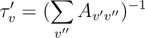
where v' and v'' are the vibrational levels of the lower and upper electronic state and A_v'v'' is the Einstein A coefficient (ns^-1) computed as

$\Delta E_{v'v''}$ is the energy difference (au) and TDM_v'v'' the transition dipole moment (au) of the transition.

For instance, for rotational states zero of the $^1\Sigma^+_g$ state and one of the $^1\Pi_u$ state:

Rotational quantum number for state 1: 0, for state 2: 1 -------------------------------------------------------------------------------- ~ Overlap matrix for vibrational wave functions for state number 1 1 1 .307535 2 1 .000000 2 2 .425936 3 1 .000000 3 2 .000000 3 3 .485199 ~ Overlap matrix for vibrational wave functions for state number 2 1 1 .279631 2 1 .000000 2 2 .377566 3 1 .000000 3 2 .000000 3 3 .429572 ~ Overlap matrix for state 1 and state 2 functions -.731192 -.617781 -.280533 .547717 -.304345 -.650599 -.342048 .502089 -.048727 ~ Transition moments over vibrational wave functions (atomic units) -.286286 -.236123 -.085294 .218633 -.096088 -.240856 -.125949 .183429 .005284 ~ Energy differences for vibrational wave functions(atomic units) 1 1 .015897 2 1 .010246 2 2 .016427 3 1 .004758 3 2 .010939 3 3 .017108 ~ Contributions to inverse lifetimes (ns-1) No degeneracy factor is included in these values. 1 1 .000007 2 1 .000001 2 2 .000001 3 1 .000000 3 2 .000001 3 3 .000000 ~ Lifetimes (in nano seconds) v tau 1 122090.44 2 68160.26 3 56017.08

Probably the most important caution when using the VIBROT program in diatomic molecules is that the number of vibrational states to compute and the accuracy obtained depends strongly on the computed surface. In the present case we compute all the curves to the dissociation limit. In other cases, the program will complain if we try to compute states which lie at energies above those obtained in the calculation of the curve.

10.1.3 A transition metal dimer: Ni₂

This section is a brief comment on a complex situation in a diatomic molecule such as Ni₂. Our purpose is to compute the ground state of this molecule. An explanation of how to calculate it accurately can be found in ref. [241]. However we will concentrate on computing the electronic states at the CASSCF level.

The nickel atom has two close low-lying configurations 3d⁸4s² and 3d⁹4s¹. The combination of two neutral Ni atoms leads to a Ni₂ dimer whose ground state has been somewhat controversial. For our purposes we commence with the assumption that it is one of the states derived from 3d⁹4s¹ Ni atoms, with a single bond between the 4s orbitals, little 3d involvement, and the holes localized in the $3d\delta$ orbitals. Therefore, we compute the states resulting from two holes on $\delta$ orbitals: $\delta\delta$ states.

We shall not go through the procedure leading to the different electronic states that can arise from these electronic configurations, but refer to the Herzberg book on diatomic molecules [243] for details. In $D_{{\infty}h}$ we have three possible configurations with two holes, since the $\delta$ orbitals can be either gerade (g) or ungerade (u): ( $\delta_g$ )^-2, ( $\delta_g$ )^-1( $\delta_u$ )^-1, or ( $\delta_u$ )^-2. The latter situation corresponds to nonequivalent electrons while the other two to equivalent electrons. Carrying through the analysis we obtain the following electronic states:

( $\delta_g$ )^-2 : $^1\Gamma_g$ , $^3\Sigma_g^-$ , $^1\Sigma_g^+$
( $\delta_u$ )^-2 : $^1\Gamma_g$ , $^3\Sigma_g^-$ , $^1\Sigma_g^+$
( $\delta_g$ )^-1( $\delta_u$ )^-1: $^3\Gamma_u$ , $^1\Gamma_u$ , $^3\Sigma_u^+$ , $^3\Sigma_u^-$ , $^1\Sigma_u^+$ , $^1\Sigma_u^-$

Next, we need to classify these electronic states in the lower symmetry D_2h, in which MOLCAS works. This is done in Table

, which relates the symmetry in $D_{{\infty}h}$ to that of D_2h. Since we have only $\Sigma^+$ , $\Sigma^-$ , and $\Gamma$ states here, the D_2h symmetries will be only A_g, A_u, B_1g, and B_1u. The table above can now be rewritten in D_2h:

( $\delta_g$ )^-2 : ( $^1{\rm A}_{g}$ + $^1{\rm B}_{1g}$ ), $^3{\rm B}_{1g}$ , $^1{\rm A}_{g}$
( $\delta_u$ )^-2 : ( $^1{\rm A}_{g}$ + $^1{\rm B}_{1g}$ ), $^3{\rm B}_{1g}$ , $^1{\rm A}_{g}$
( $\delta_g$ )^-1( $\delta_u$ )^-1: ( $^3{\rm A}_{u}$ + $^3{\rm B}_{1u}$ ), ( $^1{\rm A}_{u}$ + $^1{\rm B}_{1u}$ ), $^3{\rm B}_{1u}$ , $^3{\rm A}_{u}$ , $^1{\rm B}_{1u}$ , $^1{\rm A}_{u}$

$^1{\rm A}_{g}$ : $^1\Gamma_g$ ( $\delta_g$ )^-2, $^1\Gamma_g$ ( $\delta_u$ )^-2, $^1\Sigma_g^+$ ( $\delta_g$ )^-2, $^1\Sigma_g^+$ ( $\delta_u$ )^-2
$^1{\rm B}_{1u}$ : $^1\Gamma_u$ ( $\delta_g$ )^-1( $\delta_u$ )^-1, $^1\Sigma_u^+$ ( $\delta_g$ )^-1( $\delta_u$ )^-1
$^1{\rm B}_{1g}$ : $^1\Gamma_g$ ( $\delta_g$ )^-2, $^1\Gamma_g$ ( $\delta_u$ )^-2
$^1{\rm A}_{u}$ : $^1\Gamma_u$ ( $\delta_g$ )^-1( $\delta_u$ )^-1, $^1\Sigma_u^-$ ( $\delta_g$ )^-1( $\delta_u$ )^-1

$^3{\rm B}_{1u}$ : $^3\Gamma_u$ ( $\delta_g$ )^-1( $\delta_u$ )^-1, $^3\Sigma_u^+$ ( $\delta_g$ )^-1( $\delta_u$ )^-1
$^3{\rm B}_{1g}$ : $^3\Sigma_g^-$ ( $\delta_g$ )^-2, $^3\Sigma_g^-$ ( $\delta_u$ )^-2
$^3{\rm A}_{u}$ : $^3\Gamma_u$ ( $\delta_g$ )^-1( $\delta_u$ )^-1, $^3\Sigma_u^-$ ( $\delta_g$ )^-1( $\delta_u$ )^-1

It is not necessary to compute all the states because some of them (the $\Gamma$ states) have degenerate components. It is both possible to make single state calculations looking for the lowest energy state of each symmetry or state-average calculations in each of the symmetries. The identification of the $D_{{\infty}h}$ states can be somewhat difficult. For instance, once we have computed one $^1{\rm A}_{g}$ state it can be a $^1\Gamma_g$ or a $^1\Sigma_g^+$ state. In this case the simplest solution is to compare the obtained energy to that of the $^1\Gamma_g$ degenerate component in B_1g symmetry, which must be equal to the energy of the $^1\Gamma_g$ state computed in A_g symmetry. Other situations can be more complicated and require a detailed analysis of the wave function.

It is important to have clean d-orbitals and the SUPSym keyword may be needed to separate $\delta$ and $\sigma$ (and $\gamma$ if g-type functions are used in the basis set) orbitals in symmetry 1 (A_g). The AVERage keyword is not needed here because the $\pi$ and $\phi$ orbitals have the same occupation for $\Sigma$ and $\Gamma$ states.

Finally, when states of different multiplicities are close in energy, the spin-orbit coupling which mix the different states should be included. The CASPT2 study of the Ni₂ molecule in reference [241], after considering all the mentioned effects determined that the ground state of the molecule is a 0_g⁺ state, a mixture of the $^1\Sigma^+_g$ and $^3\Sigma^-_g$ electronic states. For a review of the spin-orbit coupling and other important coupling effects see reference [246].

10.1.4 High symmetry systems in MOLCAS

There are a large number of symmetry point groups in which MOLCAS cannot directly work. Although unusual in organic chemistry, some of them can be easily found in inorganic compounds. Systems belonging for instance to three-fold groups such as C_3v, D_3h, or D_6h, or to groups such O_h or D_4h must be computed using lower symmetry point groups. The consequence is, as in linear molecules, that orbitals and states belonging to different representations in the actual groups, belong to the same representation in the lower symmetry case, and vice versa. In the RASSCF program it is possible to prevent the orbital and configurational mixing caused by the first situation. The CLEAnup and SUPSymmetry keywords can be used in a careful, and somewhat tedious, way. The right symmetry behaviour of the RASSCF wave function is then assured. It is sometimes not a trivial task to identify the symmetry of the orbitals in the higher symmetry representation and which coefficients must vanish. In many situations the ground state wave function keeps the right symmetry (at least within the printing accuracy) and helps to identify the orbitals and coefficients. It is more frequent that the mixing happens for excited states.

The reverse situation, that is, that orbitals (normally degenerated) which belong to the same symmetry representation in the higher symmetry groups belong to different representations in the lower symmetry groups cannot be solved by the present implementation of the RASSCF program. The AVERage keyword, which performs this task in the linear molecules, is not prepared to do the same in non-linear systems. Provided that the symmetry problems mentioned in the previous paragraph are treated in the proper way and the trial orbitals have the right symmetry, the RASSCF code behaves properly.

There is a important final precaution concerning the high symmetry systems: the geometry of the molecule must be of the right symmetry. Any deviation will cause severe mixings. Figure

contains the SEWARD input for the magnesium porphirin molecule. This is a D_4h system which must be computed D_2h in MOLCAS.

For instance, the x and y coordinates of atoms C1 and C5 are interchanged with equal values in D_4h symmetry. Both atoms must appear in the SEWARD input because they are not independent by symmetry in the D_2h symmetry in which MOLCAS is going to work. Any deviation of the values, for instance to put the y coordinate to 0.681879 Å in C1 and the x to 0.681816 Å in C5 and similar deviations for the other coordinates, will lead to severe symmetry mixtures. This must be taken into account when geometry data are obtained from other program outputs or data bases.

**Figure 10.1:** Sample input of the SEWARD program for the magnesium porphirin molecule in the D_2h symmetry
$\begin{figure}{---------------------------------------------------}\end{figure}$

The situation can be more complex for some three-fold point groups such as D_3h or C_3v. In these cases it is not possible to input in the exact cartesian geometry, which depends on trigonometric relations and relies on the numerical precision of the coordinates entry. It is necessary then to use in the SEWARD input as much precision as possible and check on the distance matrix of the SEWARD output if the symmetry of the system has been kept at least within the output printing criteria.

10.1 Computing high symmetry molecules.

10.1.1 A diatomic heteronuclear molecule: NiH

10.1.2 A diatomic homonuclear molecule: C2

10.1.3 A transition metal dimer: Ni2

10.1.4 High symmetry systems in MOLCAS

10.1.2 A diatomic homonuclear molecule: C₂

10.1.3 A transition metal dimer: Ni₂